Core NLP & Deep Learning Research

The path

BPE tokenizer — how raw text becomes integers the model can consume
Attention mechanism — how tokens exchange information (Q, K, V, scaled dot-product, causal masking, multi-head)
RoPE — how the model knows token order, baked directly into attention
RMSNorm + SwiGLU — the normalization and feed-forward sublayers that make the block trainable and expressive; assembling the full "Llama block"
FlashAttention-2 — same attention math, computed in a way that doesn't blow up your GPU memory
Training dynamics — loss, gradients, why your gradient-norm graph looks the way it does
Sampling — turning output probabilities into actual text (top-k, temperature)
Stretch/research — modifying RoPE's decay behavior for "temporal memory," which is the open-ended part of CV.

Phase 1 - Byte-Pair Encoding (BPE)

The problem it solves. A neural net needs a fixed, finite vocabulary of integers to look up in an embedding table. Two naive options fail:

Word-level vocab: "unbelievable" and "unbelievably" become totally unrelated IDs; any word not seen in training is unrepresentable (out-of-vocabulary). Vocab size explodes with every language/domain.
Character-level vocab: no OOV problem, but sequences become enormous (a 500-word essay is ~2500 characters), and the model has to learn that "t-h-e" means "the" from scratch every time — wasted capacity.

BPE sits in between: it learns a vocabulary of subword chunks — common enough to be efficient, small enough to generalize. "unbelievable" might become ["un", "believ", "able"] — three tokens, each carrying real meaning, and each of those pieces can be reused for other words.

The training algorithm. This is the part people gloss over — here's the actual mechanics:

Start with your corpus, split into individual characters (or bytes — more on this below). This is your initial vocabulary.
Count every adjacent pair of symbols in the corpus. e.g. in low , the pairs are (l,o) and (o,w) .
Find the single most frequent pair across the whole corpus. Merge it into one new symbol, add it to the vocabulary.
Replace every occurrence of that pair in the corpus with the new merged symbol.
Repeat steps 2–4 until you hit your target vocab size (Llama uses 32k–128k depending on version).

That's it. It's a greedy frequency-based compression algorithm — literally adjacent in spirit to run-length/dictionary compression.

A worked toy example. Corpus: low, lower, lowest, newer, wider (imagine each word appears many times, with an end-of-word marker _ so the model can tell word boundaries apart from merges inside a word):

l o w _ (×5, from "low") l o w e r _ (×2) l o w e s t _ (×1) n e w e r _ (×6) w i d e r _ (×3)

Round 1 — count all adjacent pairs. (e, r) appears in "lower", "newer", "wider" → very frequent. Say it wins. Merge e r → er . Every e r in the corpus becomes er .

Round 2 — recount. Now (er, ) is common ( er ends three different words) — merge it into er_ .

Round 3 — (l, o) is common across "low", "lower", "lowest" — merge into lo .

Round 4 — (lo, w) — merge into low .

...and so on. After enough rounds, your vocabulary contains not just single characters but low , er_ , est_ , etc. — genuinely useful subword units, discovered purely from frequency, no linguistics involved.

Notice the order of merges matters and gets recorded as a ranked list — that ranking is the trained tokenizer.

Encoding new text (inference time). Given a new word, you don't redo the counting. You:

Split it into characters.
Look at your ranked merge list, and repeatedly apply the highest-ranked applicable merge until no more merges apply.

This is why encoding is fast — it's a lookup against a fixed ranked list, not a search.

Byte-level BPE — why Llama's tokenizer never fails. Character-level BPE has a hidden flaw: what characters do you start with? Unicode has ~150,000 code points, and you'll still hit something in production you didn't see in training (emoji, rare scripts). Llama, like GPT-2, starts from bytes instead of characters — there are only 256 possible byte values [0-255]. Any digital file, text, image, or sound in existence is just a combination of those 256 building blocks. Any string in any language becomes some sequence of bytes, so there is no such thing as an out-of-vocabulary character — worst case, an unfamiliar word just falls apart into individual bytes and gets merged less efficiently, but it's never unrepresentable. This is the detail most people with "basic knowledge" of BPE miss — it's not BPE-on-text, it's BPE-on-bytes.

One more practical detail: pre-tokenization. Before running BPE merges, Llama/GPT-style tokenizers first split text with a regex (splitting off punctuation, splitting on whitespace boundaries) so that merges never cross a word/punctuation boundary in a weird way (you don't want "dog." and "dog," to secretly merge into unrelated garbage tokens because a period followed them). BPE then runs independently within each pre-split chunk.

Where this connects forward: the output of this whole phase is just a sequence of integers (token IDs). Phase 2 starts exactly there — each integer gets looked up in an embedding table to become a vector, and that's what attention operates on.

Phase 2 - The Attention Mechanism

Attention is the mechanism that lets a static embedding become contextual. The vector for "bank" out of Phase 1's lookup table is identical whether it's a river bank or a bank account; attention is what lets each token look at every other token and pull in exactly the context it needs to disambiguate itself.

The formal mechanism: query, key, value

For every token's embedding vector x , you compute three separate linear projections — three learned weight matrices applied to the same input:

Query q = xW_Q — "what am I looking for"
Key k = xW_K — "what do I offer, as a label for matching"
Value v = xW_V — "what information do I actually contribute, once matched"

Score between query token i and key token j is their dot product q_i · k_j — geometrically, how aligned the two vectors are in the space the network learned. In matrix form, for the whole sequence at once:

scores = (Q Kᵀ) / √d_k softmax(scores) → attention weights (each row sums to 1) output = weights @ V

Why divide by √d_k ? As the vector dimension d_k grows, the dot product of two roughly-random vectors grows in magnitude too. Large raw scores push softmax into a saturated region (one score dominates, everything else gets a near-zero gradient), which destabilizes training. Dividing by √d_k keeps the score variance (how spread out the numbers get) roughly constant no matter how big you make the model — that's the entire reason it's called scaled dot-product attention.

Why Softmax Hates Huge Numbers

When those high scores are passed into a Softmax function to turn them into percentages (probabilities that sum to 100%).

Softmax uses exponents $e^x$. When you feed it extreme numbers:
- $e^{80}$ becomes an astronomically giant number.
- $e^{-80}$ becomes practically zero.
The Softmax output turns into an extreme "Winner Takes All":

Raw Scores: [82, -12, 5] Softmax: [100%, 0%, 0%]

Each token's new representation is now a weighted average of all tokens’ value vector, where the weights are dynamically computed relevance scores (attention + softmax) using previously learned projection matrices. That's the whole mechanism — everything else (multi-head, masking, RoPE) is refinement around this one operation.

A worked numeric example

Tiny 2D vectors so you can do this by hand (real heads use 64–128 dims, but the arithmetic is identical):

Token 1's query: q1 = [1, 0] . Two keys: k1 = [1, 0] , k2 = [0, 1] .

score_11 = q1·k1 = 1 score_12 = q1·k2 = 0 scaled (÷√2 ≈ 1.414): [0.707, 0] softmax([0.707, 0]) = [0.670, 0.330]

# Even if q.k = 0, the prob is still non-zero
# A dot product of 0 does NOT mean "ignore this word." It means "neutral/baseline relevance"
# Only the masking 0 are converted to -inf and 
-ve dot product is used to give even lower probability.

If the values are v1 = [2, 2] , v2 = [0, 4] :

output_1 = 0.670·[2,2] + 0.330·[0,4] = [1.34, 2.66]

Token 1's new representation is 67% value-1 and 33% value-2 — a concrete number, not a metaphor. Scaling to 128 dimensions and thousands of tokens is the same three lines of arithmetic, just bigger matrices.

Causal masking

For an autoregressive LM, token i must never see tokens j > i — otherwise it "cheats" during training by looking at the answer it's supposed to predict. Enforced by setting scores[i][j] = -∞ for all j > i , before the softmax. Since e^(-∞) = 0 , those positions get exactly zero weight. Mechanically trivial — just masking out the upper-triangular part of the score matrix — but it's the entire reason a decoder-only model like Llama can be trained in parallel on a full sequence while still behaving autoregressively at inference.

Multi-head attention

One set of Q/K/V can only learn one kind of relationship — it's one fixed set of learned projections, so it settles on whatever pattern reduces loss the most on average (often something like local proximity). Multi-head splits the model dimension into H parallel smaller attention computations — e.g. d_model = 4096 split into 32 heads of d_k = 128 each — with each head getting its own independently-learned W_Q, W_K, W_V . One head might specialize in subject-verb linking, another in coreference, another in tracking topic across long distances. Outputs get concatenated back to full width, then mixed by one more learned projection:

MultiHead(X) = Concat(head_1, ..., head_H) · W_O

Each head is running exactly the mechanism above, in parallel, on its own learned subspace.

Forward link to Phase 3: notice that nothing in this entire mechanism referenced token position. Q·K for "the cat sat" and "sat the cat" would come out identical — attention as described so far is a bag of tokens with learned relevance, blind to order. RoPE is the fix: it rotates Q and K based on position before the dot product, so position gets baked directly into the same score calculation you just learned by hand. That's next.

Phase 3 - RoPE

Nothing in attention referenced token position. RoPE closes it by rotating the query and key vectors themselves, based on where they sit in the sequence, before the dot product ever happens.

The core idea: rotation instead of addition

The obvious first idea — add a position vector to the token embedding (learned or sinusoidal absolute position embeddings, as in the original Transformer) — works, but it bakes in absolute position. The model has to separately learn that "word at position 5 relative to word at position 3" means the same thing as "word at position 105 relative to word at position 103." It never sees that generalization for free, and it struggles once you feed it sequences longer than anything seen in training.

RoPE's insight: instead of adding a position signal, rotate the query and key vectors by an angle proportional to their position. Rotations compose in exactly the way that makes relative position fall out for free.

The math

Take a 2D slice of the embedding (real RoPE splits the full dimension into many such 2D pairs — more on that below). A rotation by angle θ is the matrix:

R(θ) = [ cos θ −sin θ ] [ sin θ cos θ ]

For a token at position m , rotate its query vector by m·θ : q_m = R(mθ) q . For a token at position n , rotate its key vector by n·θ : k_n = R(nθ) k .

Now compute the score, q_m · k_n , which is q_mᵀ k_n = qᵀ R(mθ)ᵀ R(nθ) k .

Here's the one algebraic fact that makes RoPE work: rotation matrices compose by subtracting angles, R(mθ)ᵀ R(nθ) = R(nθ − mθ) = R((n−m)θ) . That's just the transpose of a rotation being the inverse rotation, combined with the fact that rotations in a plane are commutative and additive in their angle. So:

q_m · k_n = qᵀ R((n−m)θ) k

The absolute positions m and n have completely disappeared from the formula — only their difference (n−m) survives. That's exactly the property the slider demo showed you: shift both positions by the same amount, the score is untouched.

Many frequencies, not one

A real embedding isn't 2D — Llama's might be 4096-dimensional. RoPE splits it into d/2 pairs of dimensions, and gives each pair its own rotation frequency:

θ_i = base^(−2i / d), i = 0, 1, ..., d/2 − 1 (base is usually 10000)

Low-index pairs ( i small) get a large θ_i — they rotate fast per token step, so they distinguish nearby positions sharply but wrap around quickly (poor at long range). High-index pairs get tiny θ_i — they rotate slowly, barely changing over short distances, but stay distinguishable across very long spans. Stacked together across all the pairs, this is the same "multi-resolution clock" idea as the original sinusoidal position encodings — cheap fast hands for fine position, slow hands for coarse position — just applied as a rotation instead of an additive signal, which is what buys you the relative-position property above.

Where it plugs into your code

RoPE is applied to Q and K only — **never to V ** — and it's applied fresh inside every layer, right after the W_Q / W_K projections and before the QKᵀ dot product. It has no learned parameters at all; θ is fixed by the formula above, so there's nothing to train here — it's pure geometry injected into an otherwise-blind mechanism.

Forward link to your CV's "ongoing research" line:

That bullet about "modifying RoPE positional decay to simulate temporal memory" (about tweaking Rotary Position Embeddings (RoPE) so the model acts like human memory—naturally forgetting older things over time) is about deliberately breaking the pure relative-position invariance you just watched hold perfectly (What standard RoPE actually does is treat any two words that are 5 tokens apart identically, whether those two words are at the very beginning of the document (tokens #1 and #6) or way out at the end (tokens #10,000 and #10,005)). Standard RoPE does NOT guarantee that a token 10,000 steps ago gets lower attention than a token 10 steps ago. An ancient token can randomly hit a high dot-product match and hijack the attention mechanism.

Phase 4 - RMSNorm and SwiGLU

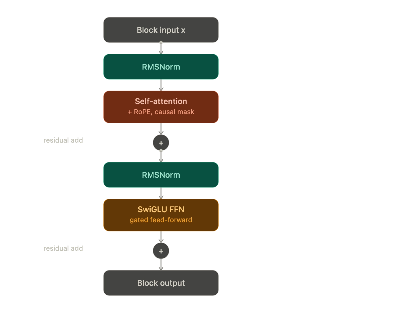Transformer block with RMSNorm, self-attention and RoPE, SwiGLU, and residual connections.

This phase is where attention finally becomes a trainable block rather than just a bare mechanism — normalization keeps the signal from blowing up or vanishing as you stack dozens of these, and the feed-forward layer is where most of the model's actual "thinking" capacity lives.That's the full block — everything from Phase 2 and 3 slots into the "self-attention" box, and everything below builds the two normalization/feed-forward pieces around it.

Why normalize at all

Stack 30+ of these blocks and activations can drift — grow layer over layer, or collapse toward zero — purely from repeated matrix multiplication, independent of whether the model is learning anything useful. That drift is exactly what shows up as unstable, spiky gradient norms during training. Normalization rescales the activation vector at fixed points in the network so every layer receives inputs of a roughly consistent magnitude, regardless of what happened in the layers before it. That's literally the mechanism behind your CV line about gradient norms stabilizing from 8.2 to 1.1 — it's not a separate trick, it's what correctly-placed norm layers do.

What is activation (x)?

If ‘x’ or ‘activation’ is entering the RMSNorm right after an Attention block, x is the token's updated contextual embedding—holding original meaning blended with the contextual information gathered from all previous tokens in the sequence.

At starts its just the vector embeddings of tokens

RMSNorm [Root Mean Square Layer Normalisation] vs LayerNorm

The original Transformer uses LayerNorm:

LayerNorm(x)_i = ((x_i − mean(x)) / sqrt(var(x) + ε)) · γ_i + β_i

It re-centers (subtracts the mean), rescales (divides by standard deviation), then applies a learned scale γ and shift β .

RMSNorm's empirical finding: the re-centering step contributes almost nothing to LayerNorm's benefit — what actually matters is controlling the vector's magnitude. So it drops the mean subtraction and the shift entirely:

RMS(x) = sqrt( (1/d) Σ x_i² ) RMSNorm(x)_i = (x_i / RMS(x)) · γ_i

One learned parameter vector ( γ , the scale), no β , no mean computation. That's fewer FLOPs per normalization call and fewer parameters — measurable savings when you're calling this twice per block, dozens of blocks deep, on every token. This is exactly why Llama (and virtually every modern open LLM) uses RMSNorm instead of LayerNorm.

Worked example. Take x = [3, 4, 0, 0] (d = 4):

RMS(x) = sqrt((9+16+0+0)/4) = sqrt(6.25) = 2.5 RMSNorm(x) = x / 2.5 = [1.2, 1.6, 0, 0] (before applying γ)

Check: RMS([1.2, 1.6, 0, 0]) = sqrt((1.44+2.56)/4) = sqrt(1.0) = 1 . No matter what the input's original scale was, the output's RMS is exactly 1 — that's the whole guarantee. If your activations had instead been x = [30, 40, 0, 0] (10× larger), you'd get the identical normalized output [1.2, 1.6, 0, 0] — RMSNorm has erased the scale, forcing every layer to receive activations in a predictable range.

Where it sits (pre-norm). Notice in the diagram that RMSNorm is applied before attention/FFN, and the residual skip carries the raw, un-normalized x_out_0 (result of previous layer) around the outside — For next block, x_out_1 = x_out_0 + Sublayer(RMSNorm(x_out_0)) , not the original "post-norm" placement. In Pre-Norm: Gradients can flow backward along the main addition path without being chopped up by normalization math. This toll-free highway is the main reason we can train massive 30+ layer models without gradients exploding or vanishing. In Post-Norm (the old way): Normalization was applied after addition. x_out = RMSNorm(x + Layer(x) This forced every single gradient through a normalization layer at every step, making deep networks very unstable and difficult to train.

SwiGLU [Swish Gated Linear Unit] : the feed-forward sublayer

One Liner : SwiGLU is a smart "gating" mechanism that uses the smooth Swish function as a flexible valve to control how much information flows through the layer.

A plain Transformer FFN is a simple two-layer MLP (Multi-Layer Perceptron) : FFN(x) = W2 · ReLU(W1 x) — expand the dimension (usually ×4), apply a nonlinearity, project back down.

SwiGLU replaces the single nonlinear path with a gated one — two parallel projections instead of one, multiplied together:

SwiGLU(x) = ( Swish(W1 x) ⊙ (W3 x) ) · W2 Swish(z) = z · sigmoid(z) (also called SiLU)

⊙ is elementwise multiplication. Read it as: W1 x produces a "gate" signal (passed through Swish), W3 x produces an independent "content" signal (left linear), and you multiply them together, unit by unit, before projecting back down with W2 . The gate isn't a fixed nonlinearity applied uniformly — it's a learned, per-unit, continuously-valued switch deciding how much of the content signal actually gets through. That's strictly more expressive than a single fixed activation function, and it's the empirical reason GLU-variant FFNs beat plain ReLU/GELU FFNs at the same parameter budget (from the "GLU Variants Improve Transformer" line of work that Llama adopted).

Worked example, one hidden unit: say (W1 x) for this unit comes out to 2 , and (W3 x) comes out to 3 .

Swish(2) = 2 · sigmoid(2) = 2 × 0.881 = 1.762 gated output = 1.762 × 3 = 5.286 ← this goes into W2

Compare to plain ReLU on the same pre-activation: ReLU(2) = 2 , with no reference to the second path at all. SwiGLU's 5.286 encodes two learned signals interacting, not one — that's the extra expressiveness per parameter.

Practical note: three weight matrices ( W1 , W3 , W2 ) instead of two means more parameters for the same hidden width, so implementations usually shrink the hidden dimension (roughly 8/3 × d_model instead of the traditional 4 × d_model ) to keep total FFN parameter count comparable to a plain MLP.

Putting the block together

Exactly what the diagram shows: RMSNorm → Attention(+RoPE) → residual add → RMSNorm → SwiGLU → residual add . Stack that N times, and after the last one, run one final RMSNorm before the output head — which is where Phase 6 and 7 pick up.

Phase 5 - FlashAttention-2

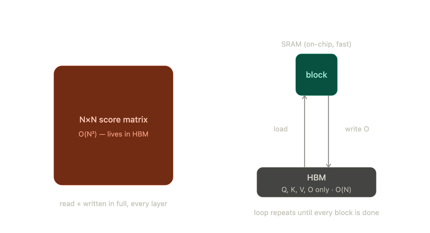Memory diagram comparing a full attention score matrix with block-based FlashAttention computation. Flash Attention is a systems-level trick: computing the *exact same* attention output while being much smarter about what touches slow memory versus fast memory.

The actual bottleneck: memory, not compute

Who is Who?

SRAM (On-Chip Memory): This is the GPU's ultra-fast, local "scratchpad." It sits right next to the compute cores inside the GPU chip. It's insanely fast, but extremely tiny (only a few megabytes).
HBM (GPU Main Memory): This is the large VRAM on your graphics card (e.g., the 80GB on an A100/H100). It holds huge models, but because it sits outside the main compute chip, data has to travel through wires to get to the processor.
We have to use HBM because normal RAM is vastly too slow, and pure SRAM is physically too small to hold giant AI models. HBM is the middle ground—big enough to fit the model, and fast enough to get the job done.

Where is the GPU waiting?

Imagine the GPU's compute cores as a super-fast calculator that can do trillions of operations per second, but it can only calculate data that is sitting in SRAM.

When running standard attention on a long sequence:

The calculator computes Q.K^T in SRAM.
SRAM is too small to keep the resulting massive N*N matrix, so it writes it out to HBM across the wire. [1 write]
Next step is Softmax. The calculator waits for the wire to fetch that matrix back from HBM into SRAM. [2 read]
It does Softmax, then writes the result back out to HBM again. [3 write]
Next step is multiplying by V. The calculator waits again for the wire to load the data back into SRAM. [4 Read and 5 Write]

The calculator finishes its math in microseconds, but spends 90% of its time idle (waiting) while data travels back and forth across the slow wire to HBM.

The trick: tiling + online softmax

FlashAttention never materializes the full N × N matrix at all. Instead:

Split Q , K , V into small blocks that fit entirely inside SRAM.
Loop over blocks of K / V . For each block, load it into SRAM once, compute the partial attention scores against the current block of Q , and accumulate a partial output — all without ever writing that intermediate score block back out to HBM.
Only the final output (size N × d , not N × N ) ever gets written back to HBM.

The one genuinely clever piece here is that softmax normally needs the whole row before it can produce any output — the denominator is a sum over every key, so how do you produce a correct result having only seen one block of keys so far? The answer is the online (streaming) softmax:

Usually, Softmax for a row of scores works like this : $\text{Softmax}(x_i) = \frac{e^{x_i - m}}{\sum e^{x_i - m}}$ Where m is the maximum score in the whole row.
Keep a running maximum m and running sum l (of exp(score − m) ) as you process each block.
Each time a new block contains a bigger score than your current running max, you don't throw away your previous partial output — you rescale it by exp(m_old − m_new) to bring it onto the new baseline, then fold in the new block's contribution.
At the very end, after all blocks are processed, divide the accumulated output by the final running sum.
Write ONLY the final answer (a small N*d matrix) back out to the slow HBM VRAM.

This produces the mathematically exact same result as computing the full softmax over all N keys at once — it's not an approximation, just a different order of operations that never requires the whole row in memory simultaneously.

What "-2" specifically improved

FlashAttention-1 already did the tiling + online-softmax trick. FlashAttention-2's gains are almost entirely about GPU utilization, not new math:

Better parallelization across sequence length. FlashAttention-1 parallelized mainly over batch size and number of attention heads. With a long sequence but small batch (common at inference, or with big models and modest batch sizes), that leaves too few independent chunks of work to keep every streaming multiprocessor on the GPU busy. FlashAttention-2 also splits work across the sequence dimension, so it stays fully occupied even with long context and small batches.

Net effect: roughly 2× throughput over FlashAttention-1, getting substantially closer to the GPU's theoretical peak FLOPs/s.

What "integrating it over SDPA" means in practice

"Integrating FlashAttention-2 over SDPA" concretely means installing the flash-attn package and explicitly using its fused CUDA kernel in your attention layer instead of relying on the default backend — same architecture, same output, but the actual memory-and-speed behavior your CV bullet describes.

Think of PyTorch’s built-in scaled_dot_product_attention (SDPA) like an automatic gear shift in a car:

What SDPA does: When you call it, PyTorch looks at your graphics card and tries to guess the fastest method to run. If your GPU supports it, it tries to use FlashAttention behind the scenes. If not, it falls back to the old, slow, memory-heavy way.
The Catch: You aren't in full control. Sometimes SDPA quietly drops back to the slow method without telling you.

Phase 6 - Loss Fn, Gradients, Gradient Norm Graph

The objective: predicting the next token

Every position in the sequence produces a vector of logits (one score per vocabulary entry) from the output head at the end of the stack. Softmax turns that into a probability distribution over the vocabulary, and the loss at that position is just:

loss_i = −log( P(actual next token | everything before it) )

This is cross-entropy — literally "how surprised was the model by the token that actually came next." If the model puts 90% probability on the correct token, loss is −log(0.9) ≈ 0.11 — small, good. If it only puts 1% probability on the correct token, loss is −log(0.01) ≈ 4.6 — large, bad. Average this over every position in the sequence and every sequence in the batch, and that scalar is what you backpropagate from — through the output head, through every block's SwiGLU and attention sublayers (chain rule flowing straight back through the residual additions you built in Phase 4), all the way to the embedding table.

Since you've already got the gradient descent / backprop mechanics down from your DPO notes, I'll skip re-deriving that and go straight to what's specific to pretraining a transformer from scratch — the optimizer choice and, most directly, the story behind that gradient-norm curve on your CV.

AdamW, briefly

Virtually every transformer is trained with AdamW: it keeps a running estimate of each parameter's gradient mean ( m ) and squared magnitude ( v ) : Detailed Info →

Think of AdamW as an ultra-smart GPS navigation system for updating a Transformer's billions of parameters during training.

1. The Core Trick: Adaptive Speed Limits (m / (sqrt{v} + epsilon))

Standard training (like basic SGD) pushes every single parameter forward using the exact same step size. AdamW is much smarter—it tracks two things for every single parameter:
1. The Direction ($m$): A running average of which way the gradient is pushing (the momentum).
2. The Wildness/Uncertainty ($v$): A running average of how huge or erratic those gradients have been.
Then it calculates your update by dividing direction by wildness: m/(sqrt{v} + epsilon)
- If a parameter's gradients are massive or wildly jumping around ($v$ is huge): AdamW hits the brakes! It shrinks the step size so the model doesn't overshoot or crash.
- If a parameter's gradients are small, steady, and consistent ($v$ is tiny): AdamW gives it a boost, letting it take a larger, confident step forward.
(The tiny epsilon is just a safety number added to the bottom so you never accidentally divide by zero!)

2. What the "W" Means (Decoupled Weight Decay)

To keep models from getting overly complex or memorizing training data, we use Weight Decay (a penalty that slowly shrinks weights toward zero).
- The Old Way (Adam + L2 Regularization): The shrinkage penalty was baked inside the gradient calculation. Because Adam rescales gradients, it accidentally messed up the shrinkage penalty for parameters with large gradients!
- The "W" Way (AdamW): AdamW decouples (separates) the shrinkage. It lets Adam handle the gradient updates, and then directly shrinks the weight by a small percentage afterward.
Old Adam: Update = Adam_Step( Gradient + Shrinkage_Penalty ) <-- Math gets distorted! AdamW: Update = Adam_Step( Gradient ) - Shrinkage_Penalty <-- Clean & direct!

AdamW is the default optimizer for Transformers because it automatically adjusts the speed limit for every single parameter based on how noisy it is, while cleanly shrinking weights in the background to prevent overfitting.

Why the gradient norm looks like the project says it does(Illustrative curve, not a literal training log — but shaped to match the 8.2 → 1.1)

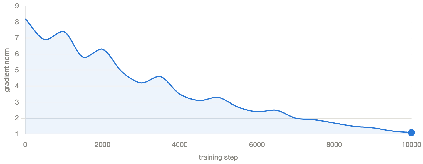Illustrative gradient-norm curve descending from roughly 8 to 1 across training steps; not a recorded training log.

Two things are producing that specific shape:

Why it's noisy and large early on. At initialization, the model's weights are close to random. Its predictions carry essentially no real structure yet, so different parts of the loss landscape can pull the parameters in poorly-aligned directions — early gradients are large and somewhat erratic. This is also exactly why training uses learning-rate warmup: start the LR near zero and ramp it up linearly over the first few hundred/thousand steps, so those large, unreliable early gradients don't take a big destabilizing step before Adam's running statistics ( m , v ) have had a chance to settle into something meaningful. Skip warmup and it's common to see the loss spike or even diverge in the first few hundred steps.

Why it settles and smooths out. Two things compound here: (1) the pre-norm residual architecture from Phase 4 keeps activation scale — and therefore gradient scale flowing backward through it — roughly consistent no matter how deep the stack is, and (2) as training progresses, the model's internal representations become more structured (attention heads and FFN units start specializing), which makes the loss surface locally smoother in the region the parameters now occupy.

The other half of the schedule: after warmup, the learning rate is typically decayed — cosine decay is the standard choice — down toward a small value over the rest of training, so updates get progressively gentler as the model approaches a good solution, avoiding overshoot late in training.

With the model actually training and producing sensible next-token probabilities, Phase 7 is about the last mile: turning those probabilities into actual generated text — . Say the word when you're ready.

Phase 7 : Sampling : Top-k and Temperature sampling

The model's output head gives you a full probability distribution over the vocabulary at each step — Phase 7 is about how you actually pick a token from that distribution to generate real text.

Why not just always pick the highest-probability token (greedy decoding)? It's deterministic and often locally "correct," but it tends to produce bland, repetitive text and can get stuck in loops on longer generations — it never lets the model deviate from its single most-confident guess, which is not how coherent, varied language actually gets produced. So generation samples randomly from the distribution instead — but the raw distribution has a very long tail of thousands of near-zero-probability tokens, and summed together that tail carries enough mass that occasionally you'd sample something incoherent purely by bad luck.

Temperature: reshaping the distribution

Standard softmax: P_i = exp(logit_i) / Σⱼ exp(logit_j) . Temperature scaling divides every logit by T first: P_i = exp(logit_i/T) / Σⱼ exp(logit_j/T) .

Worked example with three candidate logits [2, 1, 0] :

T = 1.0: softmax([2, 1, 0]) = [0.665, 0.245, 0.090] T = 0.5: softmax([4, 2, 0]) = [0.867, 0.117, 0.016] ← sharper T = 2.0: softmax([1, 0.5, 0]) = [0.506, 0.307, 0.186] ← flatter

Dividing by a T < 1 stretches the gaps between logits before exponentiating, so the exponential amplifies the leading candidate even more — the distribution sharpens toward greedy ( T → 0 recovers pure argmax). Dividing by T > 1 compresses the gaps, flattening the distribution toward uniform random sampling over the whole vocabulary as T → ∞ . Temperature never changes which token is most likely — it only changes how much more likely it is than the alternatives.

Top-k: cutting off the unreliable tail

Top-k does something temperature can't: it makes tokens structurally ineligible, regardless of how much probability mass temperature would otherwise leave them. Concretely: rank all vocabulary tokens by probability, keep only the top k , set every other token's probability to exactly zero, then renormalize the remaining k probabilities so they sum to 1 again — and sample from that truncated set. A token ranked 500th can never be sampled at k=40 no matter how high you push the temperature, because it's been removed from the pool entirely before temperature even gets applied.

The two knobs answer genuinely different questions: temperature asks "given the eligible candidates, how confidently should I favor the top one?"; top-k asks "how many candidates are even eligible to begin with?" That's why they're tuned together, not as substitutes for each other.

What "6 ablation configs for semantic coherence" means in practice

This is exactly a small grid search — something like {k=20, T=0.7} , {k=40, T=0.7} , {k=40, T=1.0} , {k=100, T=1.0} , {k=40, T=1.3} , {k=∞, T=1.0} — generating sample text under each combination and judging the output. Too low T / k and generations get repetitive and dull; too high and they drift into incoherence. "Coherence" is typically scored either heuristically (repetition rate, perplexity on held-out text) or by an LLM-as-judge comparing samples — you're literally hunting for the sweet spot the slider demo just let you feel by hand.